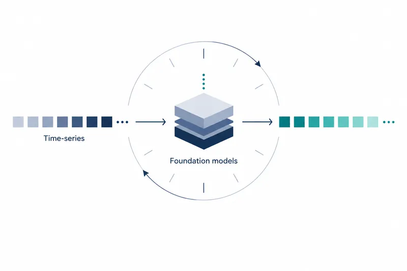
Mistral has unveiled a pretrained model family for forecasting time-ordered sensor readings or demand. Teams building equipment monitoring or demand forecasting can start with pretrained models instead of training from scratch for each dataset. The models can also run on server CPUs without a GPU.
1. Forecasting models transferable to new data
Timestral applies patterns learned from diverse time series to new data. This differs from traditional models fitted to one series or deep learning models trained from scratch for each dataset. Forecasting unseen data without additional training is called zero-shot forecasting.
2. Public benchmark rankings and comparison scope
The company said it ranked first among pretrained zero-shot models on all five metrics across three public forecasting benchmarks. These results came from a single trained model, without combining outputs from multiple models.
Results have been submitted to GIFT-Eval and TIME.
The company said its 28 million-parameter model outperformed Chronos-2, which is about 4 times larger, on these two benchmarks.
The remaining benchmark is fev-bench. A technical report with full results is planned for later release, so the rankings should be read as company-reported results at the time of the announcement.
The company said its largest model, with 209 million parameters, delivered better results at about two-thirds the size of the previous best model. It said it surpassed TimesFM-3 and Falcon-2.0 with fewer parameters. Parameter count measures model size, not actual operating costs.
3. Choosing a size means trading accuracy for latency
The models come in four sizes: 5 million, 28 million, 123 million, and 209 million parameters. They share an architecture and training method. The company says larger models improve forecasting performance, while smaller ones are faster and cheaper.
Using 8 threads on a standard server CPU, forecasting one day ahead from 3 weeks of history at 15-minute intervals took 10 milliseconds for the 5 million-parameter model and 140 milliseconds for the largest. The processor model was not specified.
In the same inference comparison, the company said the 28 million-parameter model was 5 times faster than the largest. The 123 million-parameter model used three-quarters of its latency, with a score gap within 0.2%. Measured millisecond latencies for the two middle models and the specific metric behind that score were not provided.
Choosing a smaller model reduces inference time and cost at the expense of some accuracy. Size should therefore be chosen based on forecasting errors on actual data and update frequency, rather than the largest model's ranking.
4. Handling related signals and future conditions
Multivariate forecasting predicts related series together, such as a pump's vibration, temperature, and pressure. It uses their interrelated changes rather than forecasting each sensor separately.
The output consists of 21 quantiles rather than a single predicted value. Quantiles represent values at probability positions in the forecast distribution. Teams can use this range to set alert thresholds that account for uncertainty.
Inputs can include covariates known only in the past and those with known future values, such as production schedules. Categorical values such as day of the week or equipment status are accepted directly. There is no need to convert them into numbers with arbitrary order or magnitude.
Internally, the model retains observation history in context for forecasting and distinguishes covariate roles to prevent leakage of future target values. It is first trained on synthetic data, then post-trained on a mix of real and synthetic data. The maximum input context is 32,768 time steps.
5. Applying the models to your data and operational caveats
The company released a GitHub repository for running the models on users' own data, but the announcement provided no executable code or invocation instructions.
The license was listed as Modified MIT, but detailed terms were not provided.
Mistral Forge offers options for additional training on users' own data, adjusting the training data mix, and extending the architecture.
Deployment options include on-premises infrastructure, virtual private clouds, and air-gapped environments. The full training pipeline can also be deployed on customer hardware.
Public benchmark results cannot be assumed to hold in production. If aging equipment or shifting demand changes data patterns, retraining for local conditions may be needed. Starting without additional training still leaves ongoing data management and adaptation work.
Timestral lowers the barrier to starting forecasting, but deployment decisions must weigh both model size and adaptation to field data.